
Authors: Silvia Basile, Cristian Consonni, Matteo Manca, Ludovico Boratto
Formatting converted from the ACM version of record under the supplied ACM publication authorization.
Abstract
Understanding user mobility is central to develop better transport systems that answer users’ needs. Users usually plan their travel according to their needs and preferences; however, different factors can influence their choices when traveling. In this work, we model users’ preferences, and we match their actual transport use. We use data coming from a mobility platform developed for mobile devices, whose aim is to understand the value of users’ travel time. Our first goal is to characterize the perception that users have of their mobility by analyzing their general preferences expressed before their travel time. Our approach combines dimensionality reduction and clustering techniques to provide interpretable profiles of users. Then, we perform the same task after monitoring users’ travels by doing a matching between users’ preferences and their actual behavior. Our results show that there are substantial differences between users’ perception of their mobility and their actual behavior: users overestimate their preferences for specific mobility modes, that in general, yield a lower return in terms of the worthwhileness of their trip.
CCS CONCEPTS
Applied computing → Transportation; - Information sys-
tems → Clustering.
KEYWORDS
User modeling, mobility, preferences, behavior
ACM Reference Format: Silvia Basile, Cristian Consonni, Matteo Manca, and Ludovico Boratto. 2020. Matching User Preferences and Behavior for Mobility. In Proceedings of the 31st ACM Conference on Hypertext and Social Media (HT ’20), July 13– 15, 2020, Virtual Event, USA. ACM, New York, NY, USA, 10 pages. https: //doi.org/10.1145/3372923.3404839
∗This work was developed while the author was working at Eurecat - Centre Tecnológic de Catalunya.
Permission to make digital or hard copies of all or part of this work for personal or classroom use is granted without fee provided that copies are not made or distributed for profit or commercial advantage and that copies bear this notice and the full citation on the first page. Copyrights for components of this work owned by others than ACM must be honored. Abstracting with credit is permitted. To copy otherwise, or republish, to post on servers or to redistribute to lists, requires prior specific permission and/or a fee. Request permissions from permissions@acm.org. HT ’20, July 13–15, 2020, Virtual Event, USA © 2020 Association for Computing Machinery. ACM ISBN 978-1-4503-7098-1/20/07...$15.00 https://doi.org/10.1145/3372923.3404839
1 Introduction
The advent of the Web in the last 25 years has impacted user mobility in several ways. While new forms of working and interacting with friends and family do not require to travel, people’s mobility needs are still prominent. Recent U.S. Census data indicate that the average time spent commuting has grown over the last decade [1]. Furthermore, teleworking is still an underused option, as it is generally seen as harming careers [14]. Face-to-face interactions are still needed and sought after [4, 43], and with them the need for traveling. Furthermore, the availability of portable devices and connectivity on-the-move has also changed how travelers spend their time and which activities they can perform: now, travelers can watch television [22], work [41], or play games [33, 47].
The recent Covid-19 global pandemic will redefine if and how people move, thus it is important to understand user mobility in the most comprehensive way possible. In this paper, we introduce a novel approach to model user mobility preferences and match them to typical traveler profiles. We propose a method for modeling users based on their mode-of-transport-specific as well as general preferences in terms of new characteristics of travel time: enjoyment, fitness, productivity.
In the urban context, there is a growing pressure over transport systems to respond to new needs and demands [20]: from doorto-door multi-modal trips combining public and private transport offer, to new shared mobility services (car-sharing, bike-sharing, etc.), smartphone-based ride-sharing (e.g., BlaBlaCar, Lyft, Uber) and new forms of micro-mobility (electric scooters, electric bikes, segways, etc.). This new paradigm has been labeled “Mobility as a Service” (MaaS). [19]
In this new paradigm, supporting users with intelligent transport solutions is critical. Hence, getting to know and modeling them is the first step in this direction [3]. Indeed, one might tailor these intelligent solutions based on explicit statements of the users on their preferred transport modes, by implicitly monitoring their behavior, or through a mix of both. Hence, studying the alignment between how user preferences and their actual usage of transport would allow transport operators and providers to consider the reliability of different data sources when dealing with their users. To the best of our knowledge, no work in the literature has tried to characterize and match user preferences for transport systems with their actual behavior. In this paper, we explore the difference between the perception that users have of their mobility, by analyzing their
general preferences expressed - in terms of travel modes - before their travel time and their actual transport use.
Our study covers three phases: first, we build user profiles, i.e., general descriptions of users’ based on their travel preferences; second, we build profiles using evaluation data collected after travel time; finally, we match the before- and after-travel user profiles. In this way, we want to characterize user behavior at an aggregated level, to find patterns that - together with the context provided by user profiles - can reveal useful information about users’ travel choices, taking into account different travel modes and a more complete definition of travel time.
We realized this study in the context of the Horizon 2020 project MoTiV (Mobility and Time Value), whose goal is to provide novel definitions of value of travel time (VTT) [21, 28]. Within the scope of the MoTiV project data about travelers and their journeys[1] have been collected from a dedicated mobile application, developed for the project. To model user preferences, we cluster user data and obtain an aggregated portrayal of users, i.e., user profiles [7, 8, 11, 12]. In this way, we can contextualize user preferences in general models that can be communicated to mobility stakeholders: municipalities and public administrations, transport providers, and citizens.
Specifically, the contributions of our paper are the following:
we propose a novel approach to model and profile users,
both considering preferences expressed explicitly and the monitored user behavior;
we present a matching between the preference-based profiles
and those created considering user behavior;
this is the first study that characterizes user mobility in
Europe during an extended period of time. The remainder of this paper is structured as follows. In Section 2, we review relevant literature and highlight the difference in our study with previous work. Section 3 presents the conceptual foundations of the MoTiV project, the data collected in its scope, and describes the pre-processing that we have performed prior to our analysis. Section 4 describes in detail the structure of our analysis. Finally, in Section 5, we characterize our data, and we discuss the results of our evaluation. We conclude the paper in Section 6.
2 Related Work
The analysis of human mobility patterns has been widely studied in the literature; readers can refer to Manca et al. [29] for a recent survey that considers data coming from social media, to [15] for a study by González et al. considering mobile phone data, and to Calabrese et al. [5] for an approach to extract mobility patterns from urban sensing data.
As mentioned in the Introduction, the analysis of the user behavior while planning travels is a key factor. For this reason, in [16] Goulias surveyed the existing travel behavior models. The literature has analyzed local data coming from a travel agency [31], or characterized mobility styles and travel behavior considering the answers to users surveys [25]. Nagy and Csiszar [30] studied the influencing factors of check-in time in air transportation. Zografos et al. [48] assessed user acceptance and willingness to pay for the use of multimodal journey planning systems. Katona and
1In this paper, we will use the terms “journey” and “trip” interchangeably.
Juhász [23] characterized user habits and multimodal route planning in the city of Budapest. Schrammel et al. [40] consider the challenges in behavior change by using data coming from journey planner application. Even though it does not strictly analyze user behavior, the work by Esztergár-Kiss and Csiszár [9], characterized Hungarian journey planners by considering the features that are made available to the users.
Other studies go beyond data analysis, e.g., to extract topic models from geolocation data [17], to forecast the evolution of preferences over time thanks to an hidden Markov model [46], or to provide a personalized journey planning to the users [18].
The data analysis can also produce insights that serve as input for other purposes, such as the improvement of transport service according to users’ needs [42], the promotion of changes of users’ habits [40] (e.g., the adoption of greener and healthier solutions [13]), and the improvement of journey planners and transport portals, considering their usability and the services they offer [10, 45].
Our work differs from the existing studies of user behavior that consider transport-related data, since (𝑖) our study is the first that characterizes user behavior both through explicit preferences and behavioral implicit data, (𝑖𝑖) we propose an approach to match user preferences and behavior, (𝑖𝑖𝑖) no extensive study of user behavior in mobility in several European countries exist.
3 Background
In this section, we describe the context for our study: the MoTiV project. First, we describe how it frames the concept of travel time, which is central in the transport literature to justify the choices of travelers. We then proceed to describe which data were collected during the project and how we have prepared them to perform our experiments.
3.1 Views on Value of Travel Time
Traditionally, in the transport context, the value of travel time is defined as the cost of time spent on transport, including both waiting time and actual travel time; this definition usually does not include the time spent in travel planning and searching. The value of time includes costs to consumers of personal unpaid time spent on travel and costs to businesses of paid employee time spent while traveling [27]. In MoTiV, the value of travel time is analyzed from a traveler’s perspective, assuming that time and cost savings are not always the main criteria influencing route and mode choice [24, 26]. Depending on the traveler’s transport attitude and context, other criteria such as environmental impact, comfort, or even weather conditions may influence the perceived value of a trip. In particular, MoTiV adopts the perspective that travel time can be “worth it,” i.e., it can be allocated for activities that the user finds useful, enjoyable, or productive. MoTiV shifts perspective from considering travel time as spent - or, worse, wasted - to time that can be characterized by other activities. Furthermore, this characterization is not limited by defining time as productive or unproductive time, because it is not necessarily related to its evaluation in terms of cost. Worthwhile time is independent of what can be monetized. The definition of worthwhile time encompasses multiple dimensions of travel time value from the perspective of the traveler; in particular, MoTiV
characterize users’ preferences and experiences along the three dimensions of fitness, enjoyment, and productivity [6], defined as follows (in parenthesis, we report a description of each dimension, visualized by users during data collection):
fitness measures how much the user values the fact that
when traveling they can exercise («When you walk, cycle, or even run on your travels, you are getting exercise and keeping in shape»);
enjoyment is related to how the travel can be used for fun or
relaxing activities («Relaxing or having fun: taking time to listen to music, rest or meditate; engaging in social media; observing the surroundings»);
productivity captures how much the user values the possibility of using travel time to complete some tasks, either
personal or work-related. («Using travel time to get things done, not only for work or study, but also personal things like managing home or family stuff»).
3.2 Data Collection
The data used in this paper have been collected through the Woorti[2], developed within the scope of the MoTiV project [6]. The application supports both Android and iOS devices and it is available in 11 languages. Data are inserted in the app directly by users that can register their trips at any time. Furthermore, data collection is also facilitated by dedicated data collection campaigns, coordinated by MoTiV campaign managers; these campaigns have targeted 10 European countries: Belgium, Croatia, Finland, France, Italy, Norway, Portugal, Slovakia, Spain, and Switzerland. Overall, the data considered in this paper cover a period of 8 months, from May 1st, 2019 to December, 13rd 2019. The use of the Woorti app consists of three main phases:
User preferences and experiences are encoded in two main sets of values, called worthwhileness[3] values:
generic worthwhileness values: they are a triplet of values
(𝐹, 𝐸, 𝑃) for fitness, enjoyment, and productivity, respectively. They measure how much the user values these dimension in general when traveling;
specific worthwhileness values: they are triplets of values
(𝐹, 𝐸, 𝑃) that the user is asked to assign for each specific mode of transport chosen in the onboarding phase. The transport modes that the user selects during the onboarding phase are called preferred transport modes. Specific worthwhileness values are the measure of how much the user values fitness, enjoyment, and productivity when using that particular transport mode. During the onboarding phase, the user is asked to provide both the generic and specific worthwhileness values on a scale from 1 to 100. When evaluating trips, the user is asked to provide an evaluation for each dimension of fitness, enjoyment, and productivity using a scale from low to high (low, medium, high). This difference in data collection depended on the design of the app, whose description is out of scope for this paper. For consistency with the evaluation values, we scale the onboarding values to the same three classes: low, for values in [0 − 33]; medium, [34 − 66]; and high, [67 − 100].
Table 1: User data collected during the onboarding phase. De- mographics information are optional.
Name Description and Admissible values
Overall evaluation of how much fitness, enjoyment, and productivity matter for a user’s travel experiences ([0-100])
Evaluation for each preferred mode of transport of how much fitness, enjoyment, and productivity matter for a user’s travel experiences using that mode of transport ([0-100])
(1) Onboarding: upon installing the application and registering
a new account, the user is introduced to the functionalities of the app. During this process, the user enters their travel preferences as well as, optionally, some basic demographic information. (2) Trip recording: the user can start a new trip and the Woorti
app automatically collects data in background. (3) Trip validation: when a trip is finished, the user can review
the data, validate it and insert other data regarding the trip (trip purpose, mood, etc). When validating a trip, the user must choose one leg of the trip as the reviewed leg.
Tables 1 and 2, respectively, describe the data collected from the application during the onboarding step and trip recording and validation steps. Within the application, a user can access their data through several screens and visualize and edit their profile information and trips. Furthermore, the application features a dashboard that presents to the user multiple statistics related to their validated trips, both at an individual level and by comparison with the Woorti community.
Generic worthwhileness (F, E, P)
Specific worthwhileness (F, E, P)
2The name of the app is a play on the words “worth it” referring to worthwhile travel time.
Gender Male, Female, Other Education level Basic, High school, or University Language cat, dut, eng, fin, fre, hrv, ita, nob, por, slo, spa Age range 16-19, 20-24, 25-29, 30-39, 40-49, 50-64, 65-74, 75+ Marital Status Divorced, Married, Registered partnership, Single, Widowed Labor Status Employed full-time, Employed part-time, Pensioner, Student, Unemployed
Each trip is composed of trip parts, that can be either a leg - i.e., a part of a journey when the app has detected some movement - or
3Although this diction of the word is less widespread than the more common variant “worthiness,” it is used throughout the project, so we keep it for consistency with the
project itself.
Table 2: Trip recording and evaluation data.
Name Description and admissible values
Trip id Identifier of the trip the leg refers to User id Identifier of the who performed the travel leg Leg duration Leg travel time expressed in minutes Leg distance Leg travel distance expressed in meters Mode of Mode of transport utilized; there are 37 transport different modes of transport
Transport Transport category associated to the category transport mode; there are 5 different
categories (Cycling and emerging micromobility, Private motorized, Public transport short distance, Public transport long distance, Walking and running)
3.3 Data Preprocessing
To obtain the data that we used for our analysis, we preprocessed the data performing four main tasks:
(1) data cleaning: we removed duplicate or incomplete data; (2) automatic merging of similar legs: we have automatically
merged trip legs when the following conditions where all met: 1) they belonged to the same user; 2) they had the same mode of transport; and 3) the time difference between the ending time of the first leg and the starting time of the second was below 5 minutes; (3) outlier removal: to reduce noise in our data, we eliminated
extremely long and short legs by removing legs belonging to the first and last percentile of the distribution of legs for each different transport mode - in terms of distance (leg distance) and time (leg duration). Trips containing one or more outlier legs were eliminated altogether. (4) user removal: we eliminated users that did not have any trip
left at the end of the previous steps.
4 Methods
Worthwhileness evaluation
Worthwhileness evaluation of the trip, expressed on a scale from low to high (low, medium, high)
a waiting event - that corresponds to the user not moving. When the app detects that a new trip part has started, it records the initial and final locations and timestamps. Furthermore, when creating a leg, the app infers a predicted mode of transport; within a leg, other statistics regarding trip time duration, speed and acceleration are collected. In the case of a waiting event, the app registers the average location. At the end of a trip users can review and validate the data collected. Since this requires an extra effort to the user, the app offers a set of incentives for users (e.g., personalized statistics in the app dashboard, point system, possibility of connecting points to campaign rewards) to validate as many trips as possible. This approach preserves the privacy of the user, since she can choose which trips to validate and submit to the server.
We assign a transport category to each trip based on the mode of transport of the reviewed leg; we consider this leg - selected by the user during trip validation - to be the main leg of the trip. There are five different transport categories:
(1) Cycling and emerging micromobility: comprising bikes, bike-
sharing, skates, electric scooters; (2) Private motorized: comprising cars (both as a driver and as a
passenger), car-sharing; (3) Public transport short distance: comprising buses, metro, tram,
local trains; (4) Public transport long distance: comprising long-distance buses,
high speed trains, airplanes; (5) Walking and running: comprising walking, jogging.
Our approach works in three steps: first, we model users from the onboarding and trip data by representing them as feature vectors in two separate spaces. Then, we perform dimensionality reduction and clustering to obtain general representations of users; we call the clusters that we have obtained onboarding and trip profiles, respectively. Finally, we match onboarding and trip profiles by defining a distance function between them and applying an algorithm to obtain the lowest distance assignment.
4.1 User modeling
We model each user 𝑢 ∈ 𝑈 as a vector of 18 values, i.e., 3 generic worthwhileness values and 15 specific worthwhileness values - 3 for each of the 5 transport categories; as described in Section 3.2. We define a function b : 𝑈 ↦→ 𝑉𝑏 = R[18] that models a user 𝑢 ∈ 𝑈 to their vector representation b(𝑢), by using onboarding values. Analogously, for trips we define t : 𝑈 ↦→ 𝑉𝑡 = R[18].
We build onboarding vectors in the following way: we use the 3 generic worthwhileness values; specific worthwhileness values are calculated as follows: if a user has chosen more than one preferred transport mode in a given transport category, we compute the average of the specific worthwhileness values belonging to that category. In case a user has chosen no transport mode for a given category, we use the value of zero. Trip vectors are defined similarly: we use the 3 generic worthwhileness values and, for the 15 specific ones, we average over the worthwhileness values associated with all trips that belong to the same transport category. When a user has no trips in a given transport category, we use the value of zero.[4]
4.2 Dimensionality reduction and clustering
The limitation of the possibility of evaluating one leg per-trip was designed to shorten the number of questions and effort required to the user in reporting trips. While a trip can contain several legs, the user is informed that they can report information just for that leg and that the evaluation refers to the whole trip.
To perform dimensionality reduction, we use the Uniform Manifold Approximation and Projection (UMAP) algorithm [2]. UMAP is a technique based on the assumption that data are uniformly
4The value zero, which is mapped to the class low, is also used in the case where the user has chosen the value and where no data is available. Furthermore, it is the default value for worthwhileness values - generic and specific - in the onboarding data and the trip evaluation phase.
� /|B𝑖 | and analogously for cT𝑖 .
��b∈B𝑖 [b]
distributed over a Riemannian manifold and can be modeled with a graph, which is then embedded into a low-dimension space. UMAP depends mainly on four hyperparameters:
number of neighbors: number of neighbors selected when
creating the graph structure. Small values will focus more on local structure, eventually catching noise in the data, while larger values will give a broader overview of the structure of the space;
number of components: determines the number of dimensions
the data will be embedded into. Thanks to the structure and implementation of UMAP, the number of components does not strongly affect the computational time;
minimum distance: controls how densely points will be dis-
played, and it is mainly a graphical parameter. A lower value will contribute to forming densely packed regions, and it is suggested for clustering visualization;
number of epochs: the number of training epochs to use in
the phase of optimization of the embeddings. Larger values will produce more accurate embeddings. Once the input data have been transformed through UMAP, hierarchical clustering is then performed. This algorithm of agglomerative clustering is based on both distances among data points and distances among points belonging to the same cluster [36]. We exploited different combinations of distance measures and linkage criteria in order to find a combination that could fit with our data. We perform the clustering using different values as number of target cluster, from 2 to 16, finally, we select the best clustering model using silhouette [37] and Calinski-Harabasz scores. [44]
4.3 Cluster distance measures
Once we have obtained the onboarding and trip profiles, we need to establish how to match them. Let 𝑛𝑏 and 𝑛𝑡 be the number of onboarding profiles and trip profiles, respectively. Let {𝐵𝑖 }[𝑛]𝑖=[𝑏]1 [be the]
𝑛𝑏 onboarding profiles, i.e., the clusters obtained from onboarding data: each cluster is a set of users 𝐵𝑖 = {𝑢 ∈ 𝑈 | c(b(𝑢)) = 𝑖}, where the function c(b(𝑢)) returns the index of the onboarding cluster to which the vector b(𝑢) representing the user 𝑢 belongs. Similarly, the 𝑛𝑡 trip profiles �𝑇𝑗 �𝑛𝑗=𝑡 1 [are defined as][ 𝑇][𝑗] [=] [{][𝑢] [∈] [𝑈] [|] [c][(][t][(][𝑢][))] [=]
𝑗 }. For convenience, we also define the clusters in terms of the vector representation of the users B𝑖 = {b(𝑢) ∈ 𝑉𝑏 | 𝑢 ∈ 𝐵𝑖 } and analogously for T𝑗 = {t(𝑢) ∈ 𝑉𝑡 | 𝑢 ∈ 𝑇𝑗 }.
We introduce three distance functions:
Symmetric difference distance: is the number of users that
belong to either cluster, but that are common between the cluster 𝐵𝑖 and 𝑇𝑗 :
𝑑Δ (𝐵𝑖,𝑇𝑗 ) = |𝐵𝑖 ∪ 𝑇𝑗 | −|𝐵𝑖 ∩ 𝑇𝑗 |
Jaccard distance: is the ratio between the number of users in
the symmetric difference of 𝐵𝑖 and 𝑇𝑗, over the total number of users:
𝑑𝐽 (𝐵𝑖,𝑇𝑗 ) = [|][𝐵][𝑖] [∪] [𝑇][𝑗] [| −|][𝐵][𝑖] [∩] [𝑇][𝑗] [|]
𝐵𝑖 ∪ 𝑇𝑗 |
vector representation of cluster 𝐵𝑖 and 𝑇𝑗 :
𝑑𝐶 (𝐵𝑖,𝑇𝑗 ) = ||cB𝑖 − cT𝑖 ||
where c𝐵𝑖 =
4.4 Matching algorithm
By establishing a similarity function between onboarding and trip profiles, we can solve the problem of finding an assignment between each onboarding profile and each trip profile. We can represent the problem as having a bipartite graph where each node on the left represents a user profile, and each node on the right represent a trip profile. The graph has weighted edges, where the weight over the edge between the nodes representing the onboarding profile 𝐵𝑖 and the node representing the trip profile 𝑇𝑗 is the distance between the clusters 𝐵𝑖 and 𝑇𝑗, using one of the distance measures defined above. The problem that we want to solve is then framed as finding the subset of edges that assign each node on the left to one - and only one - node on the right with the minimal overall weight.
The assignment problem can be solved by a classical algorithm called the Hungarian method or Kuhn-Munkres algorithm. This assignment algorithm starts from a feasible solution - the empty assignment being one such solution - and then it finds a progressively better one until it reaches an optimal one.
5 Experiments
In this section, we present the results of our study. We begin by describing our experimental setup. For our experiment, first, we perform some descriptive analysis on our dataset to characterize users and trips. Then, we explore several settings of parameters for the dimensionality reduction and clustering algorithm and we present some results that justify our choices for the final configuration. Finally, we describe the results of the matching between onboarding and trips profiles and we discuss them in detail.
5.1 Experimental setup
We performed our experiments on a server running Ubuntu 18.04 LTS (bionic). Our code was written Python (version 3.6) and using Jupyter notebooks[5] (modules jupyter v. 1.0.0, jupyter-core v. 4.6.1).
Data were processed using Pandas[6] pandas v. 0.24.2 and NumPy[7] (numpy v. 1.17.4). We used the UMAP Python module[8]
(umap-learn v. 0.3.10). For the cluster matching, we used the implementation of the Hungarian algorithm available via SciPy[9]
(scipy v. 1.3.2). We generated the plots using Matplotlib[10]
(matplotlib v. 3.1.2), seaborn[11] (seaborn v. 0.9.0), and Plotly[12] (plotly v. 4.5.0).
5.2 User characterization
With the Woorti app, we collected data from 3,330 users, consisting of 71,509 validated trips and 179,679 legs. After preprocessing, described in Section 3.3, our dataset contains data from 3,011 unique users, contributing a total of 50,133 validated trips and 153,553 legs.
5https://jupyter.org/ 6https://pandas.pydata.org/ 7https://numpy.org/ 8https://umap-learn.readthedocs.io/en/latest/ 9https://www.scipy.org/ 10https://matplotlib.org/ 11https://seaborn.pydata.org/ 12https://plotly.com/python/
Table 3: Number (#) and fraction expressed as a percentage (𝑓 ) of: trips by transport category (trips); users with at least one trip in that category (Users (trips)); and users which selected at least one preferred mode of transport in that cat- egory (Users (ob)).
Category
Trips Users (trips) Users (ob)
𝑓 (%) # 𝑓 (%) # 𝑓 (%)
Cycling and micro 11023 21.99 1317 43.74 2009 66.72 Private motorized 15003 29.93 1741 57.82 2153 71.50 Public long-dist 481 0.96 189 5.28 1146 38.06 Public short-dist 6097 12.16 1211 40.22 1986 65.96 Walking 17529 34.96 2124 70.54 2360 78.36
Table 3 presents the number of trips and users for each transport category. Since a user could choose multiple preferred modes of transport and perform multiple trips, the sum of users is greater than the number of unique users.
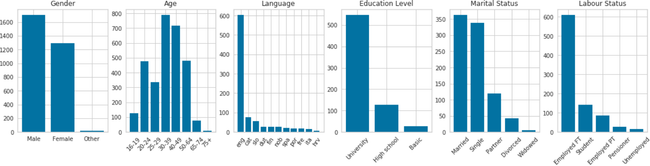
Figure 1 shows some insights about the demographics of users. More than half of the users are male, and half of the users are between 30 and 49 years old. The main language used in the application was English. Furthermore - taking into account that less than only 30% of users declared their education level, marital or labor status - 80% of users that reported the information have a university degree, 42% are married while 39% are single; 69% have a full-time job while 16% are students.
5.3 Dimensionality Reduction and Clustering: Hyperparameter Tuning
In this section, we describe the set of hyperparameters we have chosen to run the UMAP dimensionality reduction algorithm:
the number of components was set to 2, in this way we could
visualize and inspect the results of the clustering algorithm;
the minimum distance was set equal to 0, to get a better shape
of the clusters;
the number of epochs was set to 500, keeping the default
value;
for choosing the number of neighbors, we tuned this parameter by running the UMAP algorithm with values ranging
from 10 to 100, in order to explore both the local and global structure of the space in which the data were embedded. Finally, we selected 10 as the number of neighbors for the onboarding data, and 60 for the trip data. This choice is motivated not only by the intention to find a trade-off between the manifold features which are captured by the parameter, but also by looking at the final structure that seems to be already divided into groups that will facilitate the clustering algorithm.
Once we have obtained the reduced dataset for both onboarding and trip data, we run the hierarchical clustering algorithm with different combinations of the number of clusters, distance metrics, and linkage criteria. For our final results, we have chosen to use
the Euclidean distance as metric and Ward’s method as linkage criterion. The number of clusters was set to 5, with a Silhouette score of 0.68 for onboarding profiles and 0.66 for trip profiles and a Calinski-Harabasz score of 30,880 for the former and 13,478 for the latter. Moreover, we think that 5 is the minimum number of clusters needed to group the users, since we have 5 transport categories.
5.4 Profile Matching
We use the distances defined in Section 4.3 to compute the distance between each onboarding and trip profiles. We obtain 5 × 5 cost matrices, that are reported in Table 4. We run the Hungarian algorithm over these matrices and obtain a set of matching pairs of profiles. The matching calculated using the symmetric difference distance and the Jaccard distance are the same, while the matching obtained using the centroid distance are different. Using the centroid distance, closer profiles are more similar in terms of their characteristics. The best matching is computed by considering the overall cost of the assignment, not necessarily by matching the closest profiles; the optimal solution is given by the assignment for which the total distance is minimized.
5.5 Discussion
Thanks to our approach, we can describe the results of the clustering in terms of the characteristics of the users. Figure 2 represents the values for the generic and specific worthwhileness value for each transport category for the trip (top row) and onboarding (middle row) profiles. Each cell of the map contains the average worthwhile value for the corresponding factor (fitness, enjoyment, productivity) and transport category for users belonging to that profile. Each onboarding profile matches with the trip profile directly above, so the figure highlights the similarity between matched profiles. Furthermore, we are interested in studying if user preferences and evaluations are different before and after their travels. In the bottom row of Figure 2, we take the users belonging to the onboarding profiles in the middle row, and we visualize the average of the specific worthwhileness values for their trips. By comparing the middle and bottom rows, we appreciate the difference between users’ expectations - expressed before their travels - and the evaluation of the trips that they have performed. The heatmaps in the bottom row present only the specific worthwhileness values because these are the results of the evaluation of trips for a given transport mode and transport category, so there is no direct comparison for the generic worthwhileness values. We can recognize some overall common characteristics of the clusters:
Comparing specific worthwhileness values - columns 1-3
of each heatmap in Figure 2, P (productivity), E (enjoyment), and F (fitness), respectively, with general worthwhileness values - columns 4-6, GenP (productivity), GenE (enjoyment), and GenF (fitness), respectively - we see that general worthwhileness values receive an overall higher evaluation than the corresponding categories of specific worthwhileness values. This is true across all clusters and transport modes. This difference could signal a mismatch between general expectation related to transport use, with respect to more concrete prospects when asked about specific transport modes. In practice, this data may suggest that users would like to enjoy
{(𝐵1,𝑇3); (𝐵2;𝑇4); (𝐵3;𝑇1); (𝐵4;𝑇2); (𝐵5;𝑇5)} when using symmetric difference and Jaccard distance; and {(𝐵1,𝑇4); (𝐵2;𝑇3); (𝐵3;𝑇1); (𝐵4;𝑇2); (𝐵5;𝑇5)} when using centroid distance.
(a) (b)
𝐵 𝑇 1 2 3 4 5 1 1460 1247 945 1241 1109
2 1186 757 907 735 737
3 947 820 1342 1014 1174
4 1213 526 908 734 734
1 2 3 4 5 0.172 0.046 0.266 0.096 0.125
0.119 0.033 0.083 0.125 0.081
0.318 0.160 0.020 0.112 0.007
0.085 0.168 0.050 0.088 0.041
5 1412 771 811 811 | 547 | Col3 |
|---|
0.036 0.029 0.143 0.082 | 0.232 |
|---|
(c)
1 2 3 4 5 2.944 3.860 1.785 3.659 2.901
2.854 3.756 1.703 3.686 3.012
1.301 2.620 2.380 2.694 3.413
1.438 0.862 2.415 0.874 2.066
2.903 2.899 1.677 2.518 | 0.861 |
|---|
more their travel time, but when asked to relate it to actual transportation their are already lowering their expectation. We think that the reason for this mismatch merit further investigation.
productivity is, in general, lower across the board than the
enjoyment and fitness, except for the categories of Private motorized (private cars, car-sharing) and Public transport both for short and long distances - for fitness.
modes of transport belonging to the categories Walking and
running and Cycling and emerging micromobility receive a high evaluation in terms of enjoyment and fitness.
Based on the onboarding characteristics and preferred transport mode choices of the users, and with reference to Figure 2, we can describe each onboarding profile (middle row) as follows:
(1) (1[st] column) users with high values for fitness and enjoyment
while having low values for productivity. They are the active people, whose preferred modes of transport are comprised in the walking and running, cycling, and public transport categories;
(2) (2[nd] column) users with medium values for fitness and pro ductivity but high values for enjoyment. They are active people, who choose to walk and cycle, but also use their private car; (3) (3[rd] column) users with medium to low values for fitness,
high enjoyment, and medium productivity. These users walk, use their private car and local public transport, but they do no cycle or use micromobility modes of transport; (4) (4[th] column) users with medium to low values for fitness
and productivity, and medium values for enjoyment. These users have the overall lowest values in all categories. They mostly use private cars and public transport; (5) (5[th] column) users with high values for fitness, medium-to high values for enjoyment, and low values for productivity. These users use cycling and new forms of micromobility, together with private cars and public transport.
By comparing the onboarding profiles with their matched trip profile (middle and top rows), we see that across the board, the evaluation for all worthwhileness factors (fitness, enjoyment, and
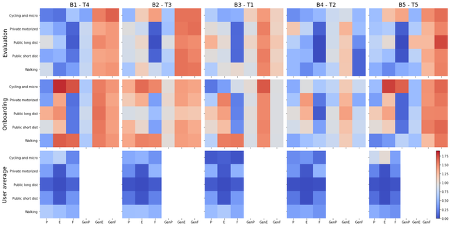
0 - corresponding to low - is blue, and 2 - corresponding to high - is red. Matching onboarding and trip profiles are one underneath the other, left to right 𝐵1 − 𝑇 4, 𝐵2 − 𝑇 3, 𝐵3 − 𝑇 1, 𝐵4 − 𝑇 2, and 𝐵5 − 𝑇 5. The heatmaps in the bottom row are 5 × 3 matrices and visualize the average of the specific worthwhileness values of the trips performed by users belonging to the onboarding profiles above.
productivity) is lower. This comparison is even starker if we consider the onboarding profile and the evaluation of trips given by the same set of users (middle and bottom rows).
Another way to quantify the differences between user expectations when planning a journey and their travel choices is to consider the alluvial diagram of Figure 3. The diagram depicts of the number of users belonging to matching profiles; overall, only 927 out of 3,011 user (31%) migrate from an onboarding profile to their matching trip profile while most (2,084, 69%) users migrate to a profile with more significant differences with respect to the profile describing their preferences. Table 5 reports the number of users belonging to either one of the matching profile pairs (𝐵𝑖,𝑇𝑗 ) and the number of users in common 𝐵𝑖 ∩ 𝑇𝑗 .
6 Conclusions
In this paper, we focused on user modeling according to their mobility and tried to understand if the preferences they explicitly express match with their behavior. To accomplish this goal, we considered data coming from a mobile application, whose goal is to understand users’ value of travel time. We proposed a user profiling approach based on dimensionality reduction and clustering techniques and applied it to the explicitly expressed user preferences and the data
Table 5: Composition of user profiles: each column presents, for each pair of matching onboarding and trip profiles (𝐵𝑖,𝑇𝑗 ) the number of users belonging to onboarding pro- files but not to the corresponding trip profile 𝐵𝑖 𝑇𝑗 , and vice versa 𝑇𝑗 𝐵𝑖 , and the users in common 𝐵𝑖 ∩ 𝑇𝑗 . The sym- metric difference between 𝐵𝑖 and 𝑇𝑗 can also be computed as Δ(𝐵𝑖,𝑇𝑗 ) = |𝐵𝑖 𝑇𝑗 | + |𝑇𝑗 𝐵𝑖 |.
(𝐵1,𝑇4) (𝐵2,𝑇3) 𝐵3,𝑇1) (𝐵4,𝑇2) (𝐵5,𝑇5)
𝐵𝑖 𝑇𝑗 865 355 320 262 282 𝑇𝑗 𝐵𝑖 376 552 627 264 265 𝐵𝑖 ∩ 𝑇𝑗 132 82 442 106 165
coming from their mobility behavior. Then, we proposed an algorithm to match the profiles, to understand how users’ intentions fit with their actual behavior.
Results show that users’ overestimate their preferences for specific mobility modes, that in general yield a lower return in terms of the worthwhileness of their trip, and that the matching between preferences and behavior reveals that the same user ends up being
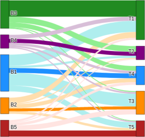
927 out of 3011 users (31%) migrate to their matching profile.
characterized in very different ways following their intentions and their actual usage of transport. This difference is even more prominent for general worthwhileness values, that are not tied to any transport mode, compared to specific worthwhileness values.
Along the dimensions of productivity, enjoyment, and fitness, that our project has introduced to characterize the value of travel time, our data shows that productivity receives lower scores across the board. Further research should focus on exploring the underlying motives of this difference, as well as to investigate the mismatch between generic and specific worthwhileness values.
This paper provides a proposal towards a more holistic evaluation of travel time that extends the traditional evaluation measured in monetary terms. We also have proposed a method to evaluate user preferences and match them to their transport usage. Describing a complete picture of the time spent while traveling, whose complexity has surged since the advent of digital technologies, could improve our understanding of how to develop the transport infrastructure in the future. This enhanced understanding can give us practical, actionable insights that could be translated into technical and policy recommendations for the next transport systems.
We plan to extend our work by considering additional dimensions associated with the features of the users, such as their gender [32], age, or provenience. Our goal is to understand if different categories of users adhere to their preferences more or less, in order to extract more actionable knowledge from the analysis of user mobility. We also plan to develop trip-ranking algorithms [34, 35, 38, 39] that are tailored around these profiles, to inject value of travel time notions into decision support systems.
Acknowledgments
This article received the support of the MoTiV project, funded from the European Union’s Horizon 2020 research and innovation programme under grant agreement No 825225 (https://motivproject.eu/)
References
[1] [n.d.]. U.S. Census Bureau Commuting. https://www.census.gov/topics/ employment/commuting/guidance/commuting.html. Accessed: 2020-02-06.
[2] Etienne Becht, Leland McInnes, John Healy, Charles-Antoine Dutertre, Im manuel WH Kwok, Lai Guan Ng, Florent Ginhoux, and Evan W Newell. 2019. Dimensionality reduction for visualizing single-cell data using UMAP. Nature biotechnology 37, 1 (2019), 38.
[3] Ludovico Boratto, Matteo Manca, Giuseppe Lugano, and Marián Gogola. 2020.
Characterizing user behavior in journey planning. Computing 102, 5 (2020), 1245–1258. https://doi.org/10.1007/s00607-019-00775-8
[4] Christina Breuer, Joachim Hüffmeier, Frederike Hibben, and Guido Hertel. 2020.
Trust in teams: A taxonomy of perceived trustworthiness factors and risk-taking behaviors in face-to-face and virtual teams. human relations 73, 1 (2020), 3–34.
[5] Francesco Calabrese, Mi Diao, Giusy Di Lorenzo, Joseph Ferreira, and Carlo Ratti.
Understanding individual mobility patterns from urban sensing data: A
mobile phone trace example. Transportation research part C: emerging technologies 26 (2013), 301–313.
[6] Yannick Cornet, Merrill Jones Barradale, João Bernardino, and Giuseppe Lugano.
Worthwhile Travel Time: Design Challenges of Capturing the User Experience by Smartphone. In 2019 Smart City Symposium Prague (SCSP). IEEE,
1–9.
[7] Danilo Dessì, Gianni Fenu, Mirko Marras, and Diego Reforgiato Recupero. 2017.
Leveraging Cognitive Computing for Multi-class Classification of E-learning Videos. In The Semantic Web: ESWC 2017 Satellite Events - ESWC 2017 Satellite Events, Portorož, Slovenia, May 28 - June 1, 2017, Revised Selected Papers (Lec- ture Notes in Computer Science), Eva Blomqvist, Katja Hose, Heiko Paulheim, Agnieszka Lawrynowicz, Fabio Ciravegna, and Olaf Hartig (Eds.), Vol. 10577. Springer, 21–25. https://doi.org/10.1007/978-3-319-70407-45
[8] Danilo Dessì, Gianni Fenu, Mirko Marras, and Diego Reforgiato Recupero. 2018.
COCO: Semantic-Enriched Collection of Online Courses at Scale with Experimental Use Cases. In Trends and Advances in Information Systems and Technologies Volume 2 [WorldCIST’18, Naples, Italy, March 27-29, 2018] (Advances in Intelligent Systems and Computing), Álvaro Rocha, Hojjat Adeli, Luís Paulo Reis, and Sandra Costanzo (Eds.), Vol. 746. Springer, 1386–1396. https://doi.org/10.1007/978-3- 319-77712-2133
[9] Domokos Esztergár-Kiss and Csaba Csiszár. [n.d.]. Multicriteria Analysis of
Hungarian Journey Planners. Periodica Polytechnica Transportation Engineering 44, 2 ([n. d.]). https://doi.org/10.3311/PPtr.8570
[10] D. Esztergár-Kiss. 2016. Optimization of multimodal travel chains. Ph.D. Dis sertation. Budapest University of Technology and Economics, Kandó Kálmán Doctoral School.
[11] Gianni Fenu and Mirko Marras. 2017. Leveraging Continuous Multi-modal
Authentication for Access Control in Mobile Cloud Environments. In New Trends in Image Analysis and Processing - ICIAP 2017 - ICIAP International Workshops, WBICV, SSPandBE, 3AS, RGBD, NIVAR, IWBAAS, and MADiMa 2017, Catania, Italy, September 11-15, 2017, Revised Selected Papers (Lecture Notes in Computer Science), Vol. 10590. Springer, 331–342. https://doi.org/10.1007/978-3-319-70742-631
[12] Gianni Fenu, Mirko Marras, and Massimiliano Meles. 2017. A learning analytics
tool for usability assessment in moodle environments. Journal of e-Learning and Knowledge Society 13, 3 (2017).
[13] Silvia Gabrielli, Paula Forbes, Antti Jylhä, Simon Wells, Miika Sirén, Samuli
Hemminki, Petteri Nurmi, Rosa Maimone, Judith Masthoff, and Giulio Jacucci.
Design challenges in motivating change for sustainable urban mobility.
Computers in Human Behavior 41 (2014), 416–423. https://doi.org/10.1016/j.chb. 2014.05.026
[14] Timothy Golden, Kimberly A Eddleston, and Gary N Powell. 2017. The impact
of teleworking on career success: A signaling-based view. In Academy of Management Proceedings, Vol. 2017. Academy of Management Briarcliff Manor, NY 10510, 14757.
[15] Marta C. González, Cesar A. Hidalgo R., and Albert-László Barabási. 2008. Un derstanding individual human mobility patterns. nature 453, 7196 (2008), 779.
[16] Konstadinos G. Goulias. 2018. Travel behavior models. In Handbook of Behavioral
and Cognitive Geography, Daniel R. Montello (Ed.). Edward Elgar Publishing Limited, USA, Chapter 5, 56–73.
[17] Samiul Hasan and Satish V. Ukkusuri. 2014. Urban activity pattern classification
using topic models from online geo-location data. Transportation Research Part C: Emerging Technologies 44 (2014), 363 – 381. https://doi.org/10.1016/j.trc.2014. 04.003
[18] Michal Jakob, Jan Hrncir, Luis Oliva, Francesco Ronzano, Pavol Zilecky, and Jason
Finnegan. 2014. Personalized Fully Multimodal Journey Planner. In Proceedings of the Twenty-first European Conference on Artificial Intelligence (Prague, Czech Republic) (ECAI’14). IOS Press, Amsterdam, The Netherlands, The Netherlands, 1225–1226. https://doi.org/10.3233/978-1-61499-419-0-1225
[19] Peraphan Jittrapirom, Valeria Caiati, Anna-Maria Feneri, Shima Ebrahimighare hbaghi, María González, and Jishnu Narayan. 2017. Mobility as a Service: A
Critical Review of Definitions, Assessments of Schemes, and Key Challenges. Urban Planning 2, 2 (2017), 13–25. https://doi.org/10.17645/up.v2i2.931
[20] Maria Kamargianni, Weibo Li, Melinda Matyas, and Andreas Schäfer. 2016. A
critical review of new mobility services for urban transport. Transportation Research Procedia 14 (2016), 3294–3303.
[21] Aleksandar Karadimce, Giuseppe Lugano, and Yannick Cornet. 2018. Modelling
the Quality of User-perceived Travel Experience. In 1st International Conference Applied Computer Technologies (ACT 2018). 142–148.
[22] Dmytro Karamshuk, Nishanth Sastry, Mustafa Al-Bassam, Andrew Secker, and
Jigna Chandaria. 2016. Take-away TV: Recharging work commutes with predictive preloading of catch-up TV content. IEEE Journal on Selected Areas in Communications 34, 8 (2016), 2091–2101.
[23] Gíza Katona and János Juhász. 2017. User habits and multimodal route planning.
Production Engineering Archives 16 (10 2017), 22–27. https://doi.org/10.30657/ pea.2017.16.05
[24] Tatiana Kováčiková, Giuseppe Lugano, and Ghadir Pourhashem. 2017. From
travel time and cost savings to value of mobility. In International Conference on Reliability and Statistics in Transportation and Communication. Springer, 35–43.
[25] Martin Lanzendorf. 2002. Mobility Styles and Travel Behavior: Application of
a Lifestyle Approach to Leisure Travel. Transportation Research Record 1807, 1 (2002), 163–173. https://doi.org/10.3141/1807-20
[26] Giuseppe Lugano, Zuzana Kurillova, Martin Hudák, and Ghadir Pourhashem.
Beyond Travel Time Savings: Conceptualizing and Modelling the Individual
Value Proposition of Mobility. In The 4th Conference on Sustainable Urban Mobility. Springer, 714–721.
[27] P.J. Mackie, S. Jara-Díaz, and A.S. Fowkes. 2001. The value of travel time savings
in evaluation. Transportation Research Part E: Logistics and Transportation Review 37, 2 (2001), 91 – 106. https://doi.org/10.1016/S1366-5545(00)00013-2 Advances in the Valuation of Travel Time Savings.
[28] Eva Malichová, Ghadir Pourhashem, Tatiana Kováčiková, and Martin Hudák.
Users’ Perception of Value of Travel Time and Value of Ridesharing Impacts
on Europeans’ Ridesharing Participation Intention: A Case Study Based on MoTiV European-Wide Mobility and Behavioral Pattern . Sustainability 12, 10 (May 2020), 1–19. https://ideas.repec.org/a/gam/jsusta/v12y2020i10p4118-d359553.html
[29] Matteo Manca, Ludovico Boratto, Victor Morell Roman, Oriol Martori i Gallissà,
and Andreas Kaltenbrunner. 2017. Using social media to characterize urban mobility patterns: State-of-the-art survey and case-study. Online Social Networks and Media 1 (2017), 56–69. https://doi.org/10.1016/j.osnem.2017.04.002
[30] Eniko Nagy and Csaba Csiszar. 2018. Revealing Influencing Factors of Check-in
Time in Air Transportation. Acta Polytechnica Hungarica 17 (2018), 225–243. https://doi.org/10.12700/APH.14.4.2017.4.13
[31] Bing Pan, Lixuan Zhang, and Kevin Smith. 2011. A Mixed-Method Study of User
Behavior and Usability on an Online Travel Agency. J. of IT & Tourism 13, 4 (2011), 353–364. https://doi.org/10.3727/109830512X13364362859975
[32] Ghadir Pourhashem and Giuseppe Lugano. 2020. Gender and Generation effects
on Perception of Value of Travel Time and Mode Choice. In Proceedings of 8th Transport Research Arena TRA 2020, April 27-30, 2020, Helsinki, Finland.
[33] Saumay Pushp, Chi Harold Liu, Fangming Liu, and Junehwa Song. 2014. Multi player gaming in public transport crowd: Opportunities and challenges. In 2014 IEEE World Forum on Internet of Things (WF-IoT). IEEE, 331–336.
[34] Guilherme Ramos and Ludovico Boratto. 2020. Reputation (In)dependence in
Ranking Systems: Demographics Influence Over Output Disparities. In Proceedings of the 43rd International ACM SIGIR Conference on Research and Development
in Information Retrieval, SIGIR 2020, Xi’an, China, July 25-30, 2020. ACM.
[35] Guilherme Ramos, Ludovico Boratto, and Carlos Caleiro. 2020. On the negative
impact of social influence in recommender systems: A study of bribery in collaborative hybrid algorithms. Information Processing & Management (2020), 102058. https://doi.org/10.1016/j.ipm.2019.102058
[36] Lior Rokach and Oded Maimon. 2005. Clustering methods. In Data mining and
knowledge discovery handbook. Springer, 321–352.
[37] Peter J Rousseeuw. 1987. Silhouettes: a graphical aid to the interpretation and
validation of cluster analysis. Journal of computational and applied mathematics 20 (1987), 53–65.
[38] João Saúde, Guilherme Ramos, Ludovico Boratto, and Carlos Caleiro. 2020. A
Robust Reputation-based Group Ranking System and its Resistance to Bribery. CoRR abs/2004.06223 (2020). arXiv:2004.06223 https://arxiv.org/abs/2004.06223
[39] João Saúde, Guilherme Ramos, Carlos Caleiro, and Soummya Kar. 2017.
Reputation-Based Ranking Systems and Their Resistance to Bribery. In 2017 IEEE International Conference on Data Mining, ICDM 2017, New Orleans, LA, USA, November 18-21, 2017, Vijay Raghavan, Srinivas Aluru, George Karypis, Lucio Miele, and Xindong Wu (Eds.). IEEE Computer Society, 1063–1068. https: //doi.org/10.1109/ICDM.2017.139
[40] Johann Schrammel, Sebastian Prost, Elke E. Mattheiss, Efthimios Bothos, and
Manfred Tscheligi. 2015. Using Individual and Collaborative Challenges in Behavior Change Support Systems: Findings from a Two-Month Field Trial of a Trip Planner Application. In Persuasive Technology - 10th International Conference, PERSUASIVE 2015, Chicago, IL, USA, June 3-5, 2015, Proceedings (Lecture Notes in Computer Science), Thomas MacTavish and Santosh Basapur (Eds.), Vol. 9072. Springer, 160–171. https://doi.org/10.1007/978-3-319-20306-515
[41] F Atiyya Shaw, Aliaksandr Malokin, Patricia L Mokhtarian, and Giovanni Circella.
It’s not all fun and games: an investigation of the reported benefits and
disadvantages of conducting activities while commuting. Travel Behaviour and Society 17 (2019), 8–25.
[42] Grzegorz Sierpiński and Marcin Staniek. 2017. Heuristic approach in a multi modal travel planner to support local authorities in urban traffic management. Transportation Research Procedia 27 (2017), 640 – 647. https://doi.org/10.1016/j. trpro.2017.12.027 20th EURO Working Group on Transportation Meeting, EWGT 2017, 4-6 September 2017, Budapest, Hungary.
[43] John B Thompson. 2020. Mediated interaction in the digital age. Theory, Culture
& Society 37, 1 (2020), 3–28.
[44] Toon Van Craenendonck and Hendrik Blockeel. 2015. Using internal validity
measures to compare clustering algorithms. Benelearn 2015 Poster presentations (online) (2015), 1–8.
[45] A. Vargas, H. Weffers, and H. V. da Rocha. 2011. Analyzing user interaction logs
to evaluate the usability of Web applications. In 2011 3rd Symposium on Web Society. 61–67. https://doi.org/10.1109/SWS.2011.6101272
[46] Feras El Zarwi, Akshay Vij, and Joan Walker. 2017. Modeling and Forecasting the
Evolution of Preferences over Time: A Hidden Markov Model of Travel Behavior. arXiv preprint arXiv:1707.09133 (2017).
[47] Nairan Zhang, Youngki Lee, Meera Radhakrishnan, and Rajesh Krishna Balan.
Gameon: P2p gaming on public transport. In Proceedings of the 13th Annual
International Conference on Mobile Systems, Applications, and Services. 105–119.
[48] Konstantinos G. Zografos, Konstantinos N. Androutsopoulos, and Eleni Apospori.
User Acceptance and Willingness to Pay for the Use of Multimodal Trip
Planning Systems. Procedia - Social and Behavioral Sciences 48 (2012), 2405 – 2414. https://doi.org/10.1016/j.sbspro.2012.06.1211 Transport Research Arena 2012.
Do you like what you are reading? Subscribe to receive updates.
Unsubscribe anytime